20. beta_tSNE.py
20.1. Description
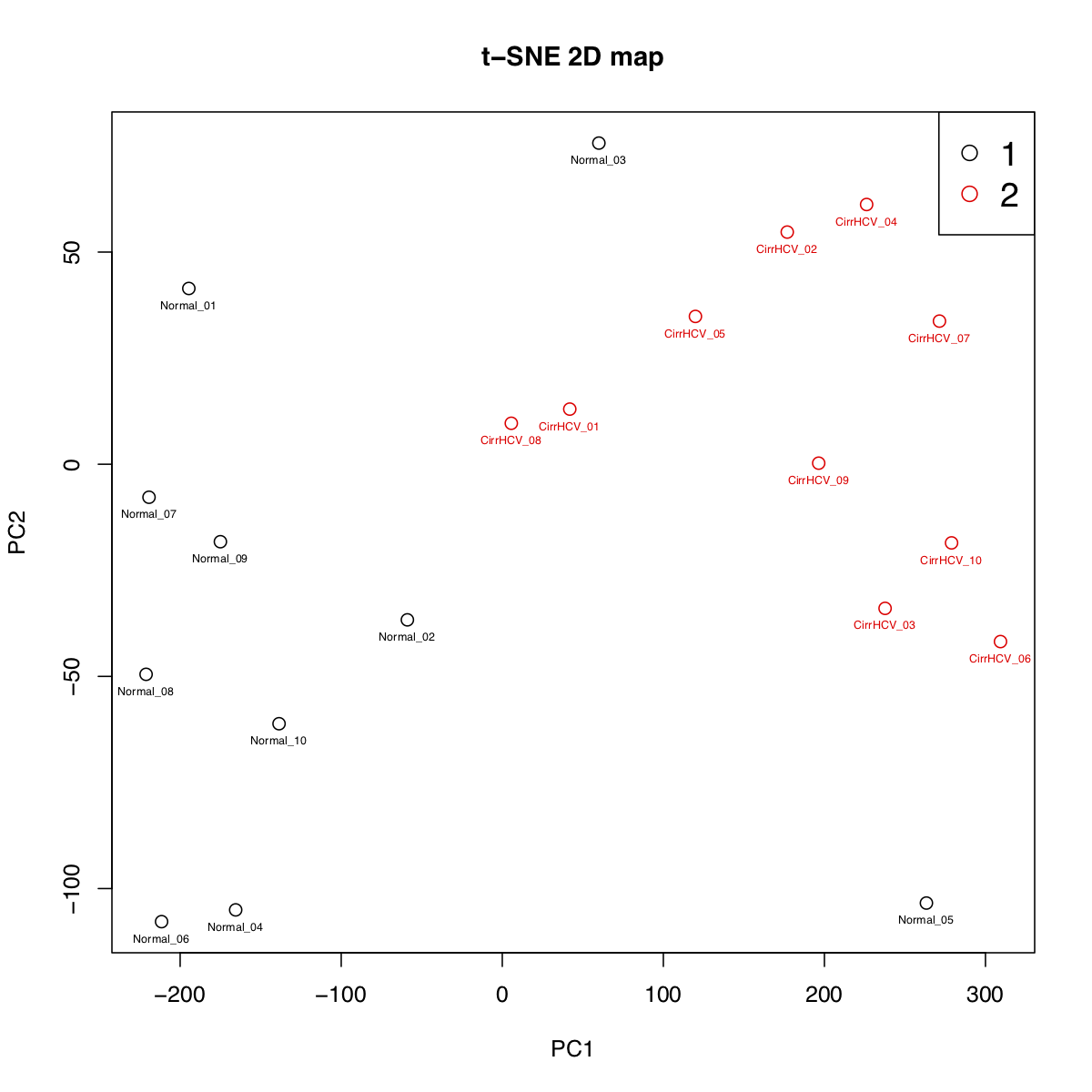
This program performs t-SNE (t-Distributed Stochastic Neighbor Embedding) analysis for samples.
Example of input data file
ID     Sample_01       Sample_02       Sample_03       Sample_04
cg_001 0.831035        0.878022        0.794427        0.880911
cg_002 0.249544        0.209949        0.234294        0.236680
cg_003 0.845065        0.843957        0.840184        0.824286
...
Example of input group file
Sample,Group
Sample_01,normal
Sample_02,normal
Sample_03,tumor
Sample_04,tumo
...
Notes
Rows with missing values will be removed
Beta values will be standardized into z scores
Only the first two components will be visualized
Different perplexity values can result in significantly different results
Even with same data and save parameters, different run might give you (slightly) different result. It is perfectly fine to run t-SNE a number of times (with the same data and parameters), and to select the visualization with the lowest value of the objective function as your final visualization.
Options:
- --version
show program’s version number and exit
- -h, --help
show this help message and exit
- -i INPUT_FILE, --input_file=INPUT_FILE
Tab-separated data frame file containing beta values with the 1st row containing sample IDs and the 1st column containing CpG IDs.
- -g GROUP_FILE, --group=GROUP_FILE
Comma-separated group file defining the biological groups of each sample. Different groups will be colored differently in the t-SNE plot. Supports a maximum of 20 groups.
- -p PERPLEXITY_VALUE, --perplexity=PERPLEXITY_VALUE
This is a tunable parameter of t-SNE, and has a profound effect on the resulting 2D map. Consider selecting a value between 5 and 50, and the selected value should be smaller than the number of samples (i.e., number of points on the t-SNE 2D map). Default = 5
- -n N_COMPONENTS, --ncomponent=N_COMPONENTS
Number of components. default=2
- --n_iter=N_ITERATIONS
The maximum number of iterations for the optimization. Should be at least 250. default=5000
- --learning_rate=LEARNING_RATE
The learning rate for t-SNE is usually in the range [10.0, 1000.0]. If the learning rate is too high, the data may look like a ‘ball’ with any point approximately equidistant from its nearest neighbors. If the learning rate is too low, most points may look compressed in a dense cloud with few outliers. If the cost function gets stuck in a bad local minimum increasing the learning rate may help. default=200.0
- -l, --label
If True, sample ids will be added underneath the data point. default=False
- -c PLOT_CHAR, --char=PLOT_CHAR
Ploting character: 1 = ‘dot’, 2 = ‘circle’. default=1
- -a PLOT_ALPHA, --alpha=PLOT_ALPHA
Opacity of dots. default=0.5
- -x LEGEND_LOCATION, --loc=LEGEND_LOCATION
Location of legend panel: 1 = ‘topright’, 2 = ‘bottomright’, 3 = ‘bottomleft’, 4 = ‘topleft’. default=1
- -o OUT_FILE, --output=OUT_FILE
The prefix of the output file.
20.2. Input files (examples)
20.3. Command
$beta_tSNE.py -i cirrHCV_vs_normal.data.tsv -g cirrHCV_vs_normal.grp.csv -o HCV_vs_normal
20.4. Output files
HCV_vs_normal.t-SNE.r
HCV_vs_normal.t-SNE.tsv
HCV_vs_normal.t-SNE.pdf