Overview¶

CpGtools package provides a number of Python programs to annotate, QC, visualize, and analyze DNA methylation data generated from Illumina HumanMethylation450 BeadChip (450K) / MethylationEPIC BeadChip (850K) array or RRBS / WGBS.

These programs can be divided into three groups:

CpG position analysis modules
CpG signal analysis modules
Differential CpG analysis modules

CpG position analysis modules¶

These modules are primarily used to analyze CpG’s genomic locations.

Name	Description
CpG_aggregation.py	Aggregate proportion values of CpGs that located in give genomic regions (eg. CpG islands, promoters, exons, etc.).
CpG_anno_position.py	Add annotation information CpGs according to their genomic coordinates.
CpG_anno_probe.py	Add annotation information to 450K/850K probes.
CpG_density_gene_centered.py	Generate the CpG density (count) profile over gene body and the up/down-stream intergenic regions.
CpG_distrb_chrom.py	Calculate the distribution of CpG over chromosomes.
CpG_distrb_gene_centered.py	Calculate the distribution of CpG over gene-centered genomic regions.
CpG_distrb_region.py	Calculate the distribution of CpG over user-specified genomic regions.
CpG_logo.py	Generate a DNA motif logo and matrices for a given set of CpGs.
CpG_to_gene.py	Assign CpGs to their putative target genes. It uses the algorithm similar to GREAT.

CpG signal analysis modules¶

These modules are primarily used to analyze CpG’s DNA methylation beta values

Name	Description
beta_PCA.py	Perform PCA (principal component analysis) for samples.
beta_jitter_plot.py	Generate jitter plot (a.k.a. strip chart) and bean plot for each sample.”
beta_m_conversion.py	Convert Beta-value into M-value or vice versa.
beta_profile_gene_centered.py	Calculate the methylation profile (i.e., average beta value) for genomic regions around genes.
beta_profile_region.py	Calculate methylation profile (i.e. average beta value) around the user-specified genomic regions.
beta_stacked_barplot.py	Create stacked barplot for each sample. The stacked barplot showing the proportions of CpGs whose beta values are falling into [0,0.25], [0.25,0.5], [0.5,0.75],[0.75,1]
beta_stats.py	Summarize basic information on CpGs located in each genomic region.
beta_tSNE.py	Perform t-SNE (t-Distributed Stochastic Neighbor Embedding) analysis for samples.
beta_topN.py	Select the top N most variable CpGs (according to standard deviation) from the input file.
beta_trichotmize.py	Use Bayesian Gaussian Mixture model to trichotmize beta values into three status: ‘Un-methylated’,’Semi-methylated’, ‘Full-methylated’, and ‘unassigned’.
beta_UMAP.py	Perform UMAP (Uniform Manifold Approximation and Projection) for samples.

Differential CpG analysis modules¶

These modules are primarily used to identify CpGs that are differentially methylated between groups

Name	Description
dmc_Bayes.py	Differential CpG analysis using the Bayesian approach. (for 450K/850K data)
dmc_bb.py	Differential CpG analysis using the beta-binomial model. (for RRBS/WGBS count data)
dmc_fisher.py	Differential CpG analysis using Fisher’s Exact Test. (for RRBS/WGBS count data)
dmc_glm.py	Differential CpG analysis using the GLM generalized liner model. (for 450K/850K data)
dmc_logit.py	Differential CpG analysis using logistic regression model. (for RRBS/WGBS count data)
dmc_nonparametric.py	Differential CpG analysis using Mann-Whitney U test for two group comparison, and the Kruskal-Wallis H-test for multiple groups comparison.
dmc_ttest.py	Differential CpG analysis using T test. (for 450K/850K data)

Installation¶

CpGtools are written in Python. Python3 (v3.5.x) is required to run all programs in CpGtools. Some programs also need R and R libraries to generate graphs and fit linear and beta-binomial models.

Prerequisites¶

Note: You need to install these tools if they are not available from your computer.

Python 3
pip3
R
R library aod (only required by dmc_bb.py)
R library beanplot (only needed by beta_jitter_plot.py)

Python Dependencies¶

Note: You do NOT need to install these packages manually, as they will be automatically installed if you use pip3 to install CpGtools.

Install CpGtools using pip3 from PyPI or github ¶

$ pip3 install cpgtools
or
$ pip3 install git+https://github.com/liguowang/cpgtools.git

Install CpGtools from source code¶

First, download the latest CpGtools, and then execute the following commands

$ tar zxf cpgtools-VERSION.tar.gz
$ cd cpgtools-VERSION
$ python3 setup.py install  #install CpGtools to the default location
or
$ python3 setup.py install --root-/home/my_pylib/  #install CpGtools to user specified location

After the installation is completed, you probably need to setup up the environment variables (Below is only an example. Change according to your system configuration)

$ export PYTHONPATH-/home/my_pylib/python3.7/site-packages:$PYTHONPATH

Upgrade CpGtools¶

$ pip3 install cpgtools --upgrade

CpGtools Release history¶

Version 1.10.0¶

Add beta_UMAP.py on 09/24/2021

Version 1.0.8¶

Fix bug for beta_tSNE.py and beta_PCA.py when sample IDs are number.

Version 1.0.7¶

Add CpG_density_gene_centered.py on 03/11/2020

Version 1.0.2¶

Add beta_tSNE.py on 07/15/2019: This program performs t-SNE (t-Distributed Stochastic Neighbor Embedding) analysis for samples.

Version 1.0.1¶

Add CpG_anno_position.py on 07/07/2019: This program annotates CpG by its genomic position using prebuilt or user-provided annotation files.

Version 1.0.0¶

Initial release

Input file and data format¶

BED file¶

BED (Browser Extensible Data) format is commonly used to describe blocks of genome. The BED format consists of one line per feature, each containing 3-12 columns of data. It is 0-based (meaning the first base of a chromosome is numbered 0). It is s left-open, right-closed. For example, the bed entry “chr1 10 15” contains the 11-th, 12-th, 13-th, 14-th and 15-th bases of chromosome-1.

BED12 file: The standard BED file which has 12 fields. Each row in this file describes a gene or an array of disconnected genomic regions. Details are described here
BED3 file: Only has the first three required fields (chrom, chromStart, chromEnd). Each row is used to represent a single genomic region where “score” and “strand” are not necessary.
BED3+ file: Has at least three columns (chrom, chromStart, chromEnd). It could have other columns, but these additional columns will be ignored.
BED6 file: Has the first six fields (chrom, chromStart, chromEnd, name, score, strand). Each row is used to represent a single genomic region and their associated scores, or in cases where “strand” information is essential.
BED6+ file: Has at least six columns (chrom, chromStart, chromEnd, name, score, stand). It could have other columns, but these additional columns will be ignored.

Proportion values¶

In bisulfite sequencing (RRBS or WGBS), the methylation level of a particular CpG or region can be represented by a “proportion” value. We define the proportion value as a pair of integers separated by comma (“,”) with the first integer (m, 0 <- m <- n) representing “number of methylated reads” and the second integer (n, n >- 0) representing “number of total reads”. for example:

0,10   1,27    2,159   #Three proportions values indicated 3 hypo-methylated loci
7,7    17,19   30,34   #Three proportions values indicated 3 hyper-methylated loci

Beta values¶

The Beta-value is a value between 0 and 1, which can be interpreted as the approximation of the percentage of methylation for a given CpG or locus. One can convert proportion value into beta value, but not vice versa. In the equation below, C is the “probe intensity” or “read count” of methylated allele, while U is the “probe intensity” or “read count” of unmethylated allele.

\[\beta=\frac{C}{U+C}, (0 \leq \beta \leq 1)\]

M values¶

The M-value is calculated as the log2 ratio of the probe intensities (or read counts) of methylated allele versus unmethylated allele. In the equation below, C is the “probe intensity” or “read count” of methylated allele, while U is the “probe intensity” or “read count” of unmethylated allele. w is the offset or pseudo count added to both denominator and numerator to avoid unexpected big changes and performing log transformation on zeros.

\[M=\log _{2}\left(\frac{C+w}{U+w}\right)\]

Convert Beta value to M value or vice versa¶

The relationship between Beta-value and M-value is shown as equation and figure:

\[\beta=\frac{2^{M}}{2^{M}+1} ; M=\log _{2}\left(\frac{\beta}{1-\beta}\right)\]

Pre-compiled datasets¶

Test datasets¶

Test dataset can be downloaded from this link

Reference gene models¶

Reference gene model files can be downloaded from this link

Annotation datasets¶

pre-built TSV file used to annotate CpG according to its 450K/850K probe ID.

MethylationEPIC_CpGtools.tsv.gz

BED files used to annotate CpG according to its genomic positions (hg19/GRCh37)

hg19_ENCODE_338TF_130Cell_E3.bed.gz

hg19_ENCODE_DNaseI_125Cells_V3.bed.gz

hg19_ENCODE_H3K27ac_11_cellLines_ChIP.bed.gz

hg19_ENCODE_H3K4me1_11_cellLines_ChIP.bed.gz

hg19_ENCODE_H3K4me3_11_cellLines_ChIP.bed.gz

hg19_ENCODE_chromHMM_states_9Cells.merge.bed.gz

hg19_FANTOM_enhancers_phase_1_and_2.bed.gz

BED files used to annotate CpG according to its genomic locations (hg38/GRCh38)

hg38_ENCODE_338TF_130Cell_E3.bed.gz

hg38_ENCODE_DNaseI_125Cells_V3.bed.gz

hg38_ENCODE_H3K27ac_11_cellLines_ChIP.bed.gz

hg38_ENCODE_H3K4me1_11_cellLines_ChIP.bed.gz

hg38_ENCODE_H3K4me3_11_cellLines_ChIP.bed.gz

hg38_ENCODE_chromHMM_states_9Cells.merge.bed.gz

hg38_FANTOM_enhancers_phase_1_and_2.bed.gz

CpG_aggregation.py¶

Description¶

Aggregate proportion values of a list of CpGs that located in give genomic regions (eg. CpG islands, promoters, exons, etc.).

Example of input file

Chrom  Start   End     score
chr1   100017748       100017749       3,10
chr1   100017769       100017770       0,10
chr1   100017853       100017854       16,21

Notes

Outlier CpG will be removed if the probability of observing its proportion value is less than p-cutoff. For example, if alpha set to 0.05, and there are 10 CpGs (n = 10) located in a particular genomic region, the p-cutoff of this genomic region is 0.005 (0.05/10). Supposing the total reads mapped to this region is 100, out of which 25 are methylated reads (i.e. regional methylation level beta = 25/100 = 0.25)

The probability of observing CpG (3,10) is : pbinom(q=3, size=10, prob=0.25) = 0.7759
The probability of observing CpG (0,10) is : pbinom(q=0, size=10, prob=0.25) = 0.05631
The probability of observing CpG (16,21) is : pbinom(q=16, size=21, prob=0.25, lower.tail=F) = 1.19e-07 (outlier)

Options¶

--version show program’s version number and exit

-h, --help show this help message and exit

-i INPUT_FILE, --input=INPUT_FILE

Input CpG file in BED format. The first 3 columns contain “Chrom”, “Start”, and “End”. The 4th column contains proportion values.

-a ALPHA_CUT, --alpha=ALPHA_CUT

The chance of mistakingly assign a particular CpG as an outlier for each genomic region. default-0.05

-b BED_FILE, --bed=BED_FILE

BED3+ file specifying the genomic regions.

-o OUT_FILE, --output=OUT_FILE

Prefix of the output file.

Input files (examples)¶

Command¶

$CpG_aggregation.py -b hg19.RefSeq.union.1Kpromoter.bed.gz  -i test_03_RRBS.bed -o out

Output¶

chr1    567292  568293  3       0       93      3       0       93
chr1    713567  714568  6       0       100     6       0       100
chr1    762401  763402  7       0       110     7       0       110
chr1    762470  763471  10      0       158     10      0       158
chr1    854571  855572  2       12      16      2       12      16
chr1    860620  861621  16      91      232     16      91      232
chr1    894178  895179  12      151     229     41      506     735

Description

Column1-3: Genome coordinates
Column4-6: numbers of “CpG”, “aggregated methyl reads”, and “aggregate total reads” after outlier filtering
Column7-9: numbers of “CpG”, “aggregated methyl reads”, and “aggregate total reads” before outlier filtering

CpG_anno_position.py¶

Description¶

This program adds annotation information to each CpG based on its genomic position.

Notes¶

Input CpG (-i) and annotation (-a) BED files must have at least three columns, and must based on the same genome assembly version
If multiple regions from the annotation BED file are overlapped with the same CpG site, their names will be concatenated together.
Since the input (-i) is a regular BED foramt file, this module can be uesd to annotate any genomic regions of interest.

Pre-computed datasets¶

hg19_ENCODE_338TF_130Cell_E3.bed.gz (File size = 108.2 MB): Transcription factor (TF) binding sites identified from ChIP-seq experiments performed by the ENCODE project. Peaks from 1264 experiments representing 338 transcription factors in 130 cell types are combined (N = 10,560,472). BED format file was downloaded from the UCSC Tabel Browser.
hg19_ENCODE_DNaseI_125Cells_V3.bed.gz (File size = 24.3 MB): DNase I hypersensitivity sites identified from ENCODE DNase-seq experiments. Peaks from 125 cell types are combined (N = 1,867,665). BED format file was downloaded from the UCSC Tabel Browser.
hg19_ENCODE_chromHMM_states_9Cells.merge.bed.gz (File size = 32.7 MB): Chromatin State Segmentation by chromHMM from ENCODE. Chromatin states across 9 cell types (GM12878, H1-hESC, K562, HepG2, HUVEC, HMEC, HSMM, NHEK, NHLF) were learned by integrating 9 factors (CTCF, H3K27ac, H3K27me3, H3K36me3, H3K4me1, H3K4me2, H3K4me3, H3K9ac, H4K20me1 ) plus input. A total of 15 states were identified, include: State-1 (Active Promoter), state-2 (Weak Promoter), state-3 (Inactive/poised Promoter), state-4 and 5 (Strong enhancer), state-6 and 7 (Weak/poised enhancer), state-8 (insulator), state-9 (Transcriptional transition), state-10 (Transcriptional elongation), state-11 (Weak transcribed), state-12 (Polycomb-repressed), state-13 (Heterochromatin or low signal), state-14 and 15 (Repetitive/Copy Number Variation). The Original chromatin state BED file was downloaded from the UCSC Tabel Browser.
hg19_FANTOM_enhancers_phase_1_and_2.bed.gz: PHANTOM5 human permissive enhancers downloaded from here.
hg19_ENCODE_H3K4me1_11_cellLines_ChIP.bed.gz (File size = 12.2 MB): H3K4me1 (marker of active and primed enhancer) peaks identified from ENCODE histone ChIP-seq experiments. Peaks from 11 cell types (GM12878, H1-hESC, HMEC, HSMM, HUVEC, HeLaS3, HepG2, K562, Monocytes-CD14+_RO01746, NHEK, NHLF) are combined (N = 1,435,550)
hg19_ENCODE_H3K4me3_11_cellLines_ChIP.bed.gz (File size = 4.5 MB): H3K4me3 (marker of promoter) peaks identified from ENCODE histone ChIP-seq experiments. Peaks from 11 cell types (GM12878, H1-hESC, HMEC, HSMM, HUVEC, HeLaS3, HepG2, K562, Monocytes-CD14+_RO01746, NHEK, NHLF) are combined (N = 525,824)
hg19_ENCODE_H3K27ac_11_cellLines_ChIP.bed.gz (File size = 5.7 MB): H3K27ac (marker of active enhancer) peaks identified from ENCODE histone ChIP-seq experiments. Peaks from 11 cell types (GM12878, H1-hESC, HMEC, HSMM, HUVEC, HeLaS3, HepG2, K562, Monocytes-CD14+_RO01746, NHEK, NHLF) are combined (N = 665,650)

These BED files were lifted over to hg38/GRCh38 using CrossMap. The hg38-based annotation files are available from here

Options¶

--version show program’s version number and exit

-h, --help show this help message and exit

-i INPUT_FILE, --input_file=INPUT_FILE

Input CpG file in BED3+ format.

-a ANNO_FILE, --annotation=ANNO_FILE

Input annotation file in BED3+ format.

-w WINDOW_SIZE, --window=WINDOW_SIZE

Size of window centering on the middle-point of each genomic region defined in the annotation BED file (i.e., window_size*0.5 will be extended to up- and down-stream from the middle point of each genomic region). default=100

-o OUT_FILE, --output=OUT_FILE

The prefix of the output file.

-l, --header If True, the first row of input CpG file is header. default=False

Input files (examples)¶

Command¶

$CpG_anno_position.py  -l -a hg19_ENCODE_338TF_130Cell_E3.bed.gz -i test_01.hg19.bed6 -o output

Output files¶

output.anno.txt

$ head -5 output.anno.txt
#Chrom Start   End     Name    Beta    Strand  hg19_ENCODE_338TF_130Cell_E3.bed
chr1   10847   10848   cg26928153      0.8965  +       N/A
chr1   10849   10850   cg16269199      0.7915  +       N/A
chr1   15864   15865   cg13869341      0.9325  +       N/A
chr1   534241  534242  cg24669183      0.7941  +       FOXA2,MNT

CpG_anno_probe.py¶

Description¶

This program adds comprehensive annotation information to each 450K/850K array probe ID. It will add 17 columns to the original input data file. These 17 columns include (from left to right):

Header Name	Description
hg19_pos	The genomic position of the CpG on human genome assembly hg19 (or GRCh37)
hg38_pos	The genomic position of the CpG on human genome assembly hg38 (or GRCh38).
strand	Strand of the CpG. Value - “R” (reverse strand) or “F” (forward strand).
geneSymbol	Genes the CpG has been assigned to. “N/A” indicates no genes were found. This is retrieved from the Illumina MethylationEpic v1.0 B4 manifest file.
CpGisland	The CpG island (CGI) that overlaps with this CpG. “N/A” indicates no CGIs were found.
with_450K	Boolean indicating whether this CpG probe is also included in 450K. “0” - No, “1”- Yes.
SNP_ID	SNPs (rsID) that are close to this CpG. Multiple SNPs are separated by “;”. “N/A” indicates no SNPs were found.
SNP_distance	The nucleotide distances between SNPs and the CpG.
SNP_MAF	The minor allele frequencies (MAF) of SNPs.
Cross_Reactive	Boolean (“0” - No, “1”- Yes) indicating whether this CpG could be affected by cross-hybridization or underlying genetic variation as reported by this paper.
ENCODE_TF_ChIP	Transcription factor (TF) binding sites identified from ChIP-seq experiments performed by the ENCODE project. Peaks from 1264 experiments representing 338 transcription factors in 130 cell types are combined (N = 10,560,472). BED format file was downloaded from the UCSC Tabel Browser, and a detailed description is provided here.
ENCODE_DNaseI	DNase I hypersensitivity sites identified from ENCODE DNase-seq experiments. Peaks from 125 cell types are combined (N - 1,867,665). BED format file was downloaded from the UCSC Table Browser, and a detailed description is provided here.
ENCODE_H3K27ac_ChIP	H3K27ac peaks identified from ENCODE histone ChIP-seq experiments. Peaks from 11 cell types (GM12878, H1-hESC, HMEC, HSMM, HUVEC, HeLaS3, HepG2, K562, Monocytes-CD14+_RO01746, NHEK, NHLF) are combined (N = 665,650)
ENCODE_H3K4me1_ChIP	H3K4me1 peaks identified from ENCODE histone ChIP-seq experiments. Peaks from 11 cell types (GM12878, H1-hESC, HMEC, HSMM, HUVEC, HeLaS3, HepG2, K562, Monocytes-CD14+_RO01746, NHEK, NHLF) are combined (N = 1,435,550)
ENCODE_H3K4me3_ChIP	H3K4me3 peaks identified from ENCODE histone ChIP-seq experiments. Peaks from 11 cell types (GM12878, H1-hESC, HMEC, HSMM, HUVEC, HeLaS3, HepG2, K562, Monocytes-CD14+_RO01746, NHEK, NHLF) are combined (N = 525,824)
ENCODE_chromHMM	Chromatin State Segmentation by chromHMM from ENCODE. Chromatin states across 9 cell types (GM12878, H1-hESC, K562, HepG2, HUVEC, HMEC, HSMM, NHEK, NHLF) were learned by computationally by integrating 9 factors (CTCF, H3K27ac, H3K27me3, H3K36me3, H3K4me1, H3K4me2, H3K4me3, H3K9ac, H4K20me1 ) plus input. A total of 15 states were identified, include: State-1 (Active Promoter), state-2 (Weak Promoter), state-3 (Inactive/poised Promoter), state-4 and 5 (Strong enhancer), state-6 and 7 (Weak/poised enhancer), state-8 (insulator), state-9 (Transcriptional transition), state-10 (Transcriptional elongation), state-11 (Weak transcribed), state-12 (Polycomb-repressed), state-13 (Heterochromatin or low signal), state-14 and 15 (Repetitive/Copy Number Variation). Orignal chromatin state BED file was downloaded from UCSC Table Browser, and detailed description is provided here.
FANTOM_enhancer	PHANTOM5 human enhancers downloaded from here.

Notes¶

For peaks identified from ENCODE ChIP-seq and DNase-seq (ENCODE_TF_ChIP, ENCODE_H3K27ac_ChIP, ENCODE_H3K4me1_ChIP, ENCODE_H3K4me3_ChIP, and ENCODE_DNaseI), we require the probe must be located in the 100 bp window centered on the middle of the peak.

Options¶

--version show program’s version number and exit

-h, --help show this help message and exit

-i INPUT_FILE, --input_file=INPUT_FILE

Input data file (Tab-separated) with a certain column containing 450K/850K array CpG IDs. This file can be a regular text file or compressed file (.gz, .bz2).

-a ANNO_FILE, --annotation=ANNO_FILE

Annotation file. This file can be a regular text file or compressed file (.gz, .bz2).

-o OUT_FILE, --output=OUT_FILE

Prefix of the output file.

-p PROBE_COL, --probe_column=PROBE_COL

The number specifying which column contains probe IDs. Note: the column index starts with 0. default-0.

-l, --header Input data file has a header row.

Input files (examples)¶

Command¶

# probe IDs are located in the 4th column (-p 3)

$CpG_anno_probe.py -p 3 -l -a MethylationEPIC_CpGtools.tsv -i test_01.hg19.bed6 -o output

or (take gzipped files as input)

$CpG_anno_probe.py -p 3 -l -a MethylationEPIC_CpGtools.tsv.gz -i test_01.hg19.bed6.gz -o output

@ 2019-06-28 09:12:41: Read annotation file "../epic/MethylationEPIC_CpGtools.tsv" ...
@ 2019-06-28 09:12:52: Add annotation information to "test_01.hg19.bed6" ...

Output files¶

output.anno.txt

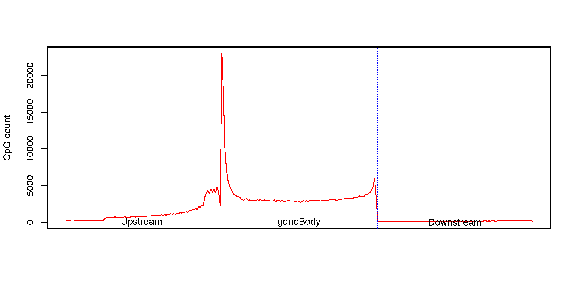
CpG_density_gene_centered.py¶

Description¶

This program calculates the CpG density (count) profile over gene body as well as its up- down-stream regions. It is useful to visualize how CpGs are distributed around genes.

Specifically, the up-stream region, gene region (from TSS to TES) and down-stream region will be equally divided into 100 bins, then CpG count was aggregated over a total of 300 bins from 5’ to 3’ (upstream bins, gene bins, downstrem bins).

Options¶

--version show program’s version number and exit

-h, --help show this help message and exit

-i INPUT_FILE, --input_file=INPUT_FILE

BED file specifying the C position. This BED file should have at least three columns (Chrom, ChromStart, ChromeEnd). Note: the first base in a chromosome is numbered 0. This file can be a regular text file or compressed file (.gz, .bz2).

-r GENE_FILE, --refgene=GENE_FILE

Reference gene model in standard BED6+ format.

-d DOWNSTREAM_SIZE, --downstream=DOWNSTREAM_SIZE

Maximum extension size from TES (transcription end site) to down-stream to define the “downstream intergenic region (DIR)”. Note: (1) The actual used DIR size can be smaller because the extending process could stop earlier if it reaches the boundary of another nearby gene. (2) If the actual used DIR size is smaller than cutoff defined by “-c/–SizeCut”, the gene will be skipped. default=2000 (bp)

-u UPSTREAM_SIZE, --upstream=UPSTREAM_SIZE

Maximum extension size from TSS (transcription start site) to up-stream to define the “upstream intergenic region (UIR)”. Note: (1) The actual used UIR size can be smaller because the extending process could stop earlier if it reaches the boundary of another nearby gene. (2) If the actual used UIR size is smaller than cutoff defined by “-c/–SizeCut”, the gene will be skipped. default=2000 (bp)

-c MINIMUM_SIZE, --SizeCut=MINIMUM_SIZE

The minimum gene size. Gene size is defined as the genomic size between TSS and TES, including both exons and introns. default=200 (bp)

-o OUT_FILE, --output=OUT_FILE

The prefix of the output file.

Input files (examples)¶

Command¶

$ python3 CpG_density_gene_centered.py -r hg19.RefSeq.union.bed  -i 850K_probe.hg19.bed3 -o CpG_density
@ 2020-03-11 14:57:10: Reading CpG file: "850K_probe.hg19.bed3"
@ 2020-03-11 14:57:14: Reading reference gene model: "hg19.RefSeq.union.bed"
@ 2020-03-11 14:57:14: Calculating CpG density ...
@ 2020-03-11 14:57:15: Wrting data to : "CpG_density.tsv"
@ 2020-03-11 14:57:15: Running R script to: 'CpG_density.r'
null device
         1

Output files¶

CpG_density.tsv
CpG_density.r
CpG_density.pdf

CpG_distrb_chrom.py¶

Description¶

This program calculates the distribution of CpG over chromosomes

Options¶

--version show program’s version number and exit

-h, --help show this help message and exit

-i INPUT_FILES, --input_files=INPUT_FILES

Input CpG file(s) in BED3+ format. Multiple BED files should be separated by “,” (eg: “-i file_1.bed,file_2.bed,file_3.bed”). BED file can be a regular text file or compressed file (.gz, .bz2). The barplot figures will NOT be generated if you provide more than 12 samples (bed files). [required]

-n FILE_NAMES, --names=FILE_NAMES

Shorter and meaningful names to label samples. Should be separated by “,” and match CpG BED files in number. If not provided, basenames of CpG BED files will be used to label samples. [optional]

-s CHROM_SIZE, --chrom-size=CHROM_SIZE

Chromosome size file. Tab or space separated text file with two columns: the first column is chromosome name/ID, the second column is chromosome size. This file will determine: (1) which chromosomes are included in the final bar plots, so do NOT include ‘unplaced’, ‘alternative’ contigs in this file. (2) The order of chromosomes in the final bar plots. [required]

-o OUT_FILE, --output=OUT_FILE

The prefix of the output file. [required]

Input files (examples)¶

Command¶

$ chrom_distribution.py -i 450K_probe.hg19.bed3.gz,850K_probe.hg19.bed3.gz -n 450K,850K \
  -s hg19.chrom.sizes -o chromDist

Output files

chromDist.txt
chromDist.r
chromDist.CpG_total.pdf
chromDist.CpG_percent.pdf
chromDist.CpG_perMb.pdf

Total CpG count per chromosome

CpG percent on each chromosome (normalized to total CpGs)

CpG per Mb (normalized to chromosome size)

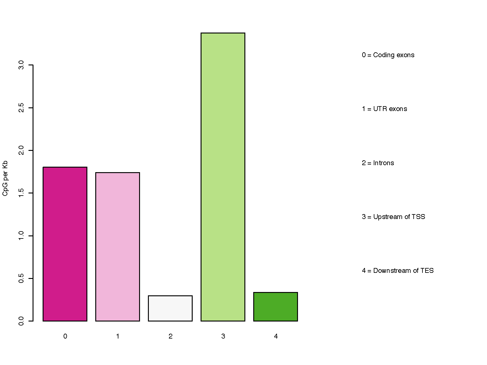
CpG_distrb_gene_centered.py¶

Description¶

This program calculates the distribution of CpG over gene-centered genomic regions including ‘Coding exons’, ‘UTR exons’, ‘Introns’, ‘ Upstream intergenic regions’, and ‘Downsteam intergenic regions’.

Notes

Please note, a particular genomic region can be assigned to different groups listed above, because most genes have multiple transcripts, and different genes could overlap on the genome. For example, an exon of gene A could be located in an intron of gene B. To address this issue, we define the priority order as below:

Coding exons
UTR exons
Introns
Upstream intergenic regions
Downstream intergenic regions

Higher-priority group override the low-priority group. For example, if a certain part of an intron is overlapped with an exon of other transcripts/genes, the overlapped part will be considered as exon (i.e., removed from intron) since “exon” has higher priority.

Options¶

--version show program’s version number and exit

-h, --help show this help message and exit

-i INPUT_FILE, --input_file=INPUT_FILE

BED file specifying the C position. This BED file should have at least three columns (Chrom, ChromStart, ChromeEnd). Note: the first base in a chromosome is numbered 0. This file can be a regular text file or compressed file (.gz, .bz2).

-r GENE_FILE, --refgene=GENE_FILE

Reference gene model in standard BED-12 format (https://genome.ucsc.edu/FAQ/FAQformat.html#format1).

-d DOWNSTREAM_SIZE, --downstream=DOWNSTREAM_SIZE

Size of down-stream intergenic region w.r.t. TES (transcription end site). default=2000 (bp)

-u UPSTREAM_SIZE, --upstream=UPSTREAM_SIZE

Size of up-stream intergenic region w.r.t. TSS (transcription start site). default=2000 (bp)

-o OUT_FILE, --output=OUT_FILE

The prefix of the output file.

Input files (examples)¶

Command¶

$ CpG_distrb_gene_centered.py -i 850K_probe.hg19.bed3.gz -r hg19.RefSeq.union.bed.gz -o geneDist

Output files¶

geneDist.tsv
geneDist.r
geneDist.pdf

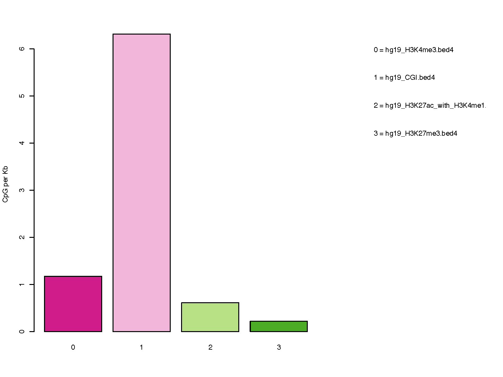
CpG_distrb_region.py¶

Description¶

This program calculates the distribution of CpG over user-specified genomic regions.

Notes

A maximum of ten BED files (define ten different genomic regions) can be analyzed together.
The order of BED files is important (i.e., considered as “priority order”). Overlapped genomic regions will be kept in the BED file with the highest priority and removed from BED files of lower priorities. For example, users provided 3 BED files via “-i promoters.bed,enhancers.bed,intergenic.bed”, then if an enhancer region is overlapped with promoters, the overlapped part will be removed from “enhancers.bed”.
BED files can be regular or compressed by ‘gzip’ or ‘bz’.

Options¶

--version show program’s version number and exit

-h, --help show this help message and exit

-i CPG_FILE, --cpg=CPG_FILE

BED file specifying the C position. This BED file should have at least three columns (Chrom, ChromStart, ChromeEnd). Note: the first base in a chromosome is numbered 0. This file can be a regular text file or compressed file (.gz, .bz2).

-b BED_FILES, --bed=BED_FILES

List of comma separated BED files specifying the genomic regions.

-o OUT_FILE, --output=OUT_FILE

The prefix of the output file.

Input files (examples)¶

850K_probe.hg19.bed3.gz Input bed file of 850K probe
hg19_CGI.bed4 CpG islands
hg19_H3K4me3.bed4 Promoters
hg19_H3K27ac_with_H3K4me1.bed4 Bivalent promoters
hg19_H3K27me3.bed4 Heterochromatin regions

Command¶

# check the distribution of 850K probes in 4 genomic regions (CpG islands, Promoters,
# Bivalent promoters, and Heterochromatin regions)

$CpG_distrb_region.py -i 850K_probe.hg19.bed3.gz -b  hg19_H3K4me3.bed4,hg19_CGI.bed4,\
 hg19_H3K27ac_with_H3K4me1.bed4,hg19_H3K27me3.bed4 -o regionDist

Output files¶

regionDist.tsv
regionDist.r
regionDist.pdf

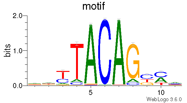
CpG_logo.py¶

Description¶

This program generates a DNA motif logo for a given set of CpGs. To answer the question of “what is the genomic context for a given list of CpGs ?”. This program first extracts genomic sequences around C position, and then generate motif matrices include:

position frequency matrix (PFM)
position probability matrix (PPM)
position weight matrix (PWM)
MEME format matrix
Jaspar format matrix

It also generates motif logo using weblogo

Notes

input BED file must have strand information.

Options¶

--version show program’s version number and exit

-h, --help show this help message and exit

-i INPUT_FILE, --input_file=INPUT_FILE

BED file specifying the C position. This BED file should have at least six columns (Chrom, ChromStart, ChromeEnd, name, score, strand). Note: Must provide correct strand information. This file can be a regular text file or compressed file (.gz, .bz2).

-r GENOME_FILE, --refgenome=GENOME_FILE

Reference genome seqeunces in FASTA format. Must be indexed using the samtools “faidx” command.

-e EXTEND_SIZE, --extend=EXTEND_SIZE

Number of bases extended to up- and down-stream. default=5 (bp)

-n MOTIF_NAME, --name=MOTIF_NAME

Motif name. default=motif

-o OUT_FILE, --output=OUT_FILE

The prefix of the output file.

Input files (examples)¶

Human reference genome sequences in FASTA format: hg19.fa.gz and hg38.fa.gz
450_CH.hg19.bed.gz

Command¶

$CpG_logo.py -i 450_CH.hg19.bed.gz -r hg19.fa -o 450_CH

Output files¶

450_CH.logo.fa
450_CH.logo.jaspar
450_CH.logo.meme
450_CH.logo.pfm
450_CH.logo.ppm
450_CH.logo.pwm
450_CH.logo.logo.pdf

CpG_to_gene.py¶

Description¶

This program annotates CpGs by assigning them to their putative target genes. It follows the “Basal plus extension rules” used by GREAT.

Basal regulatory domain is a user-defined genomic region around the TSS (transcription start site). By default, from TSS upstream 5 Kb to TSS downstream 1 Kb is considered as the gene’s basal regulatory domain. When defining a gene’s basal regulatory domain, the other nearby genes are ignored (which means different genes’ basal regulatory domain can be overlapped.)

Extended regulatory domain is a genomic region that is further extended from basal regulatory domain in both directions to the nearest gene’s basal regulatory domain but no more than the maximum extension (specified by ‘-e’, default - 1000 kb) in one direction. In other words, the “extension” stops when it reaches other genes’ “basal regulatory domain” or the extension limit, whichever comes first.

Basal regulatory domain and Extended regulatory domain are illustrated in below diagram.

Notes

Which genes are assigned to a particular CpG largely depends on gene annotation. A “conservative” gene model (such as Refseq curated protein-coding genes) is recommended.
In the refgene file, multiple isoforms should be merged into a single gene.

Description¶

This program annotates CpGs by assigning them to their putative target genes. Follows the “Basel plus extension” rules used by GREAT(http://great.stanford.edu/public/html/index.php)

Basal regulatory domain: is a user-defined genomic region around the TSS (transcription start site). By default, from TSS upstream 5kb to TSS downstream 1Kb is considered as the gene’s basal regulatory domain. When defining a gene’s “basal regulatory domain”, the other nearby genes will be ignored (which means different genes’ basal regulatory domains can be overlapped.)

Extended regulatory domain: The gene regulatory domain is extended in both directions to the nearest gene’s “basal regulatory domain” but no more than the maximum extension (default = 1000 kb) in one direction.

Notes¶

Which genes are assigned to a particular CpG largely depends on gene annotation. A “conservative” gene model (such as Refseq curated protein coding genes) is recommended.

In the gene model, multiple isoforms should be merged into a single gene.

Options¶

Options:

`--version`	show program’s version number and exit
`-h, --help`	show this help message and exit
`-i INPUT_FILE, --input-file=INPUT_FILE`
	BED3+ file specifying the C position. BED3+ file could be a regular text file or compressed file (.gz, .bz2). [required]
`-r GENE_FILE, --refgene=GENE_FILE`
	Reference gene model in BED12 format (https://genome.ucsc.edu/FAQ/FAQformat.html#format1). “One gene one transcript” is recommended. Since most genes have multiple transcripts; one can collapse multiple transcripts of the same gene into a single super transcript or select the canonical transcript.
`-u BASAL_UP_SIZE, --basal-up=BASAL_UP_SIZE`
	Size of extension to upstream of TSS (used to define gene’s “basal regulatory domain”). default=5000 (bp)
`-d BASAL_DOWN_SIZE, --basal-down=BASAL_DOWN_SIZE`
	Size of extension to downstream of TSS (used to define gene’s basal regulatory domain). default=1000 (bp)
`-e EXTENSION_SIZE, --extension=EXTENSION_SIZE`
	Size of extension to both up- and down-stream of TSS (used to define gene’s “extended regulatory domain”). default=1000000 (bp)
`-o OUT_FILE, --output=OUT_FILE`
	Prefix of the output file. Two additional columns will be appended to the original BED file with the last column indicating “genes whose extended regulatory domain are overlapped with the CpG”, the 2nd last column indicating “genes whose basal regulatory domain are overlapped with the CpG”. [required]

Input files (examples)¶

Command¶

$ CpG_to_gene.py -i  850K_probe.hg19.bed3.gz -r hg19.RefSeq.union.bed.gz -o output

Output files¶

output.associated_genes.txt

$ head output.associated_genes.txt

#The last column contains genes whose extended regulatory domain are overlapped with the CpG
#The 2nd last column contains genes whose basal regulatory domain are overlapped with the CpG
#"//" indicates no genes are found
chr1   10524   10525   DDX11L1 //
chr1   10847   10848   DDX11L1 //
chr1   10849   10850   DDX11L1 //
chr1   15864   15865   //      MIR6859-1;DDX11L1
chr1   18826   18827   MIR6859-1       //
chr1   29406   29407   WASH7P;MIR1302-2        //
chr1   29424   29425   WASH7P;MIR1302-2        //
...

beta_PCA.py¶

Description¶

This program performs PCA (principal component analysis) for samples.

Example of input data file

ID     Sample_01       Sample_02       Sample_03       Sample_04
cg_001 0.831035        0.878022        0.794427        0.880911
cg_002 0.249544        0.209949        0.234294        0.236680
cg_003 0.845065        0.843957        0.840184        0.824286
...

Example of input group file

Sample,Group
Sample_01,normal
Sample_02,normal
Sample_03,tumor
Sample_04,tumo
...

Notes

Rows with missing values will be removed
Beta values will be standardized into z scores
Only the first two components will be visualized
Variance% explained by each component will be printed to screen

Options:

`--version`	show program’s version number and exit
`-h, --help`	show this help message and exit
`-i INPUT_FILE, --input_file=INPUT_FILE`
	Tab-separated data frame file containing beta values with the 1st row containing sample IDs and the 1st column containing CpG IDs.
`-g GROUP_FILE, --group=GROUP_FILE`
	Comma-separated group file defining the biological groups of each sample. Different groups will be colored differently in the PCA plot. Supports a maximum of 20 groups.
`-n N_COMPONENTS, --ncomponent=N_COMPONENTS`
	Number of components. default=2
`-l, --label`	If True, sample ids will be added underneath the data point. default=False
`-c PLOT_CHAR, --char=PLOT_CHAR`
	Ploting character: 1 = ‘dot’, 2 = ‘circle’. default=1
`-a PLOT_ALPHA, --alpha=PLOT_ALPHA`
	Opacity of dots. default=0.5
`-x LEGEND_LOCATION, --loc=LEGEND_LOCATION`
	Location of legend panel: 1 = ‘topright’, 2 = ‘bottomright’, 3 = ‘bottomleft’, 4 = ‘topleft’. default=1
`-o OUT_FILE, --output=OUT_FILE`
	The prefix of the output file.

Input files (examples)¶

Command¶

$beta_PCA.py -i cirrHCV_vs_normal.data.tsv -g cirrHCV_vs_normal.grp.csv -o HCV_vs_normal

Output files¶

HCV_vs_normal.PCA.r
HCV_vs_normal.PCA.tsv
HCV_vs_normal.PCA.pdf

beta_UMAP.py¶

Description¶

This program performs UMAP (Uniform Manifold Approximation and Projection) non-linear dimension reduction.

Example of input data file

ID     Sample_01       Sample_02       Sample_03       Sample_04
cg_001 0.831035        0.878022        0.794427        0.880911
cg_002 0.249544        0.209949        0.234294        0.236680
cg_003 0.845065        0.843957        0.840184        0.824286
...

Example of input group file

Sample,Group
Sample_01,normal
Sample_02,normal
Sample_03,tumor
Sample_04,tumo
...

Notes

Rows with missing values will be removed
Beta values will be standardized into z scores
Only the first two components will be visualized

Options:

`--version`	show program’s version number and exit
`-h, --help`	show this help message and exit
`-i INPUT_FILE, --input_file=INPUT_FILE`
	Tab-separated data frame file containing beta values with the 1st row containing sample IDs and the 1st column containing CpG IDs.
`-g GROUP_FILE, --group=GROUP_FILE`
	Comma-separated group file defining the biological groups of each sample. Different groups will be colored differently in the 2-dimensional plot. Supports a maximum of 20 groups.
`-n N_COMPONENTS, --ncomponent=N_COMPONENTS`
	Number of components. default=2
`--nneighbors=N_NEIGHBORS`
	This parameter controls the size of the local neighborhood UMAP will look at when attempting to learn the manifold structure of the data. Low values of ‘–nneighbors’ will force UMAP to concentrate on local structure, while large values will push UMAP to look at larger neighborhoods of each point when estimating the manifold structure of the data. Choose a value from [2, 200]. default=15
`--min-dist=MIN_DISTANCE`
	This parameter controls how tightly UMAP is allowed to pack points together. Choose a value from [0, 1). default=0.2
`-l, --label`	If True, sample ids will be added underneath the data point. default=False
`-c PLOT_CHAR, --char=PLOT_CHAR`
	Ploting character: 1 = ‘dot’, 2 = ‘circle’. default=1
`-a PLOT_ALPHA, --alpha=PLOT_ALPHA`
	Opacity of dots. default=0.5
`-x LEGEND_LOCATION, --loc=LEGEND_LOCATION`
	Location of legend panel: 1 = ‘topright’, 2 = ‘bottomright’, 3 = ‘bottomleft’, 4 = ‘topleft’. default=1
`-o OUT_FILE, --output=OUT_FILE`
	The prefix of the output file.

Input files (examples)¶

Command¶

$beta_UMAP.py -i cirrHCV_vs_normal.data.tsv -g cirrHCV_vs_normal.grp.csv -o cirrHCV_vs_normal -l

Output files¶

cirrHCV_vs_normal.UMAP.r
cirrHCV_vs_normal.UMAP.tsv
cirrHCV_vs_normal.UMAP.pdf

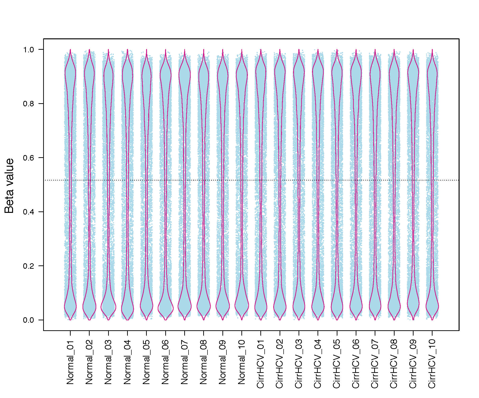
beta_jitter_plot.py¶

Description¶

This program generates jitter plot (a.k.a. strip chart) and bean plot for each sample (column)

Example of input

CpG_ID  Sample_01       Sample_02       Sample_03       Sample_04
cg_001  0.831035        0.878022        0.794427        0.880911
cg_002  0.249544        0.209949        0.234294        0.236680
cg_003  0.845065        0.843957        0.840184        0.824286

Notes

User must install the beanplot R library.
Please name your sample IDs (such as “Sample_01”, “Sample_02” in the above example) using only “letters” [a-z, A-Z], “numbers” [0-9], and “_”; and your sample ID must start with a letter.

Options¶

--version show program’s version number and exit

-h, --help show this help message and exit

-i INPUT_FILE, --input_file=INPUT_FILE

Tab-separated data frame file containing beta values with the 1st row containing sample IDs and the 1st column containing CpG IDs.

-f FRACTION, --fraction=FRACTION

The fraction of total data points (CpGs) used to generate jitter plot. Decrease this number if the jitter plot is over-crowded. default=0.5

-o OUT_FILE, --output=OUT_FILE

The prefix of the output file.

Input files (examples)¶

test_05_TwoGroup.tsv

Command¶

$beta_jitterPlot.py -f 1 -i test_05_TwoGroup.tsv.gz -o Jitter

Output files¶

Jitter.r
Jitter.pdf

beta_m_conversion.py¶

Description¶

Convert Beta-value into M-value or vice vers

Example of input (beta)

CpG_ID Sample_01 Sample_02 Sample_03 Sample_04 cg_001 0.831035 0.878022 0.794427 0.880911 cg_002 0.249544 0.209949 0.234294 0.236680 cg_003 0.845065 0.843957 0.840184 0.824286

Options¶

--version show program’s version number and exit

-h, --help show this help message and exit

-i INPUT_FILE, --input_file=INPUT_FILE

Tab-separated data frame file containing beta values with the 1st row containing sample IDs and the 1st column containing CpG IDs. This file can be a regular text file or compressed file (.gz, .bz2).

-d DATA_TYPE, --dtype=DATA_TYPE

Input data type either “Beta” or “M”.

-o OUT_FILE, --output=OUT_FILE

The output file.

Input file (example)¶

test_08.tsv.gz

Command¶

$ beta_m_conversion.py  -i test_08.tsv -d Beta -o test_08_M.tsv

Output¶

$ head -5 test_08_M.tsv
cg_ID  TCGA-BC-A10Q    TCGA-BC-A10R    TCGA-BC-A10S    TCGA-BC-A10T    TCGA-BC-A10U
cg00000029     -0.9127840676229807     -0.6635535075463712     -0.9389653708375745     -1.1786876012968779     -0.6217264255944122
cg00000165     -2.4833534763405667     -2.3330364850204406     -2.858145170950326      -2.914508967160336      -2.3645896606652745
cg00000236     2.478873972561897       3.0777336083377693      2.6760378499862143      3.04301970048709        2.7096166677505145
cg00000289     0.9943771370790748      0.13339998728363872     0.5981994318909333      1.2402989291699527      1.432741941887314

beta_profile_gene_centered.py¶

Description¶

This program calculates the methylation profile (i.e., average beta value) for genomic regions around genes. These genomic regions include:

5’UTR exon
CDS exon
3’UTR exon,
first intron
internal intron
last intron
up-stream intergenic
down-stream intergenic

Example of input (BED6+)

chr22   44021512        44021513        cg24055475      0.9231  -
chr13   111568382       111568383       cg06540715      0.1071  +
chr20   44033594        44033595        cg21482942      0.6122  -

Options¶

--version show program’s version number and exit

-h, --help show this help message and exit

-i INPUT_FILE, --input_file=INPUT_FILE

BED6+ file specifying the C position. This BED file should have at least 6 columns (Chrom, ChromStart, ChromeEnd, Name, Beta_value, Strand). BED6+ file can be a regular text file or compressed file (.gz, .bz2).

-r GENE_FILE, --refgene=GENE_FILE

Reference gene model in standard BED12 format (https://genome.ucsc.edu/FAQ/FAQformat.html#format1). “Strand” column must exist in order to decide 5’ and 3’ UTRs, up- and down-stream intergenic regions.

-d DOWNSTREAM_SIZE, --downstream=DOWNSTREAM_SIZE

Size of down-stream genomic region added to gene. default=2000 (bp)

-u UPSTREAM_SIZE, --upstream=UPSTREAM_SIZE

Size of up-stream genomic region added to gene. default=2000 (bp)

-o OUT_FILE, --output=OUT_FILE

The prefix of the output file.

Command¶

$beta_profile_gene_centered.py -i test_02.bed6.gz  -r hg19.RefSeq.union.bed.gz -o gene_profile

Output files¶

gene_profile.txt
gene_profile.r
gene_profile.pdf

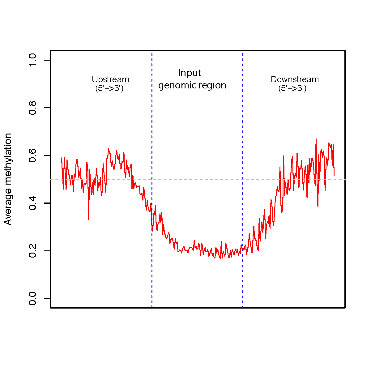
beta_profile_region.py¶

Description¶

This program calculates methylation profile (i.e. average beta value) around the user-specified genomic regions.

Example of input

# BED6 format (INPUT_FILE)
chr22   44021512        44021513        cg24055475      0.9231  -
chr13   111568382       111568383       cg06540715      0.1071  +
chr20   44033594        44033595        cg21482942      0.6122  -

# BED3 format (REGION_FILE)
chr1    15864   15865
chr1    18826   18827
chr1    29406   29407

Options¶

--version show program’s version number and exit

-h, --help show this help message and exit

-i INPUT_FILE, --input_file=INPUT_FILE

BED6+ file specifying the C position. This BED file should have at least six columns (Chrom, ChromStart, ChromeEnd, Name, Beta_value, Strand). BED6+ file can be a regular text file or compressed file (.gz, .bz2).

-r REGION_FILE, --region=REGION_FILE

BED3+ file of genomic regions. This BED file should have at least three columns (Chrom, ChromStart, ChromeEnd). If the 6-th column does not exist, all regions will be considered as on “+” strand.

-d DOWNSTREAM_SIZE, --downstream=DOWNSTREAM_SIZE

Size of extension to downstream. default=2000 (bp)

-u UPSTREAM_SIZE, --upstream=UPSTREAM_SIZE

Size of extension to upstream. default=2000 (bp)

-o OUT_FILE, --output=OUT_FILE

The prefix of the output file.

Input files (examples)¶

Command¶

$beta_profile_region.py -r hg19.RefSeq.union.1Kpromoter.bed.gz -i test_02.bed6.gz -o region_profile

Output files¶

region_profile.txt
region_profile.r
region_profile.pdf

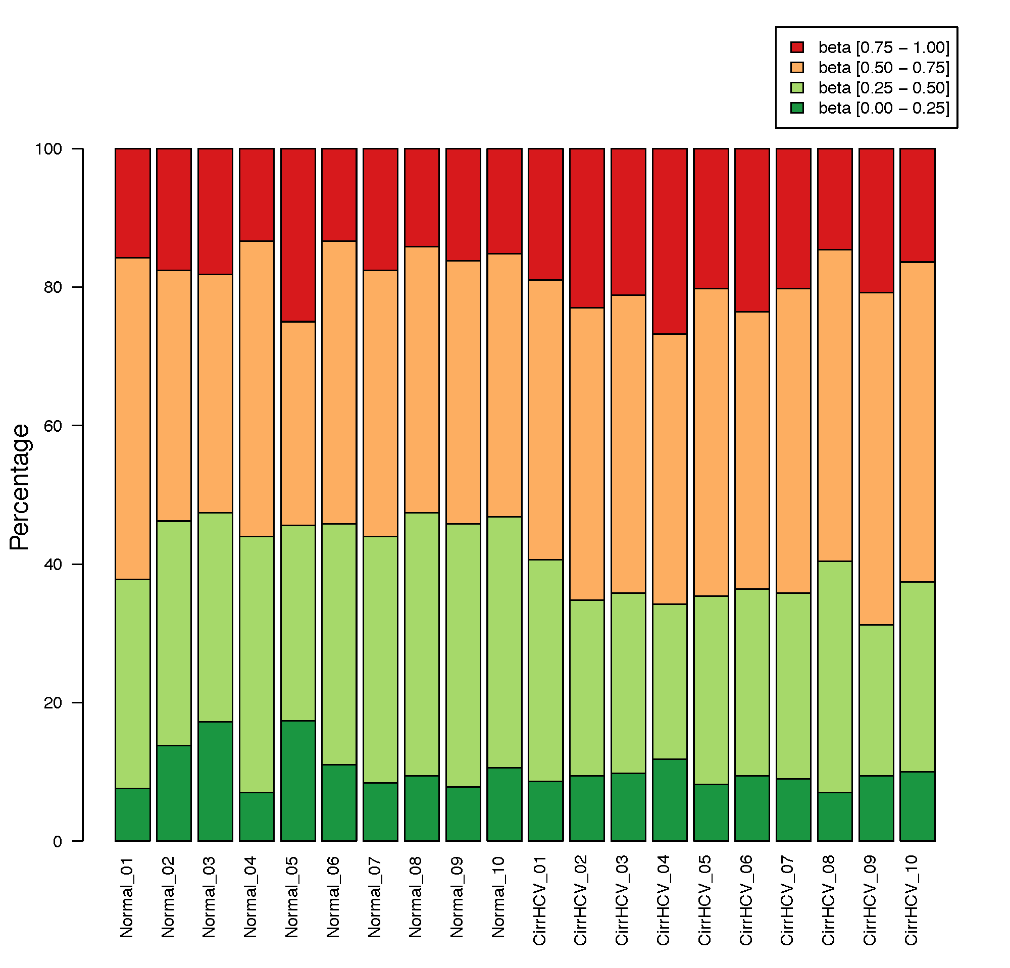
beta_stacked_barplot.py¶

Description¶

This program creates stacked barplot for each sample. The stacked barplot showing the proportions of CpGs whose beta values are falling into these four ranges:

[0.00, 0.25] #first quantile
[0.25, 0.50] #second quantile
[0.50, 0.75] #third quantile
[0.75, 1.00] #forth quantile

Example of input file

CpG_ID  Sample_01       Sample_02       Sample_03       Sample_04
cg_001  0.831035        0.878022        0.794427        0.880911
cg_002  0.249544        0.209949        0.234294        0.236680

Notes

Please name your sample IDs (such as “Sample_01”, “Sample_02” in the above example) using only “letters” [a-z, A-Z], “numbers” [0-9], and “_”; and your sample ID must start with a letter.

Options¶

Options:

`--version`	show program’s version number and exit
`-h, --help`	show this help message and exit
`-i INPUT_FILE, --input_file=INPUT_FILE`
	Data frame file containing beta values with the 1st row containing sample IDs and the 1st column containing CpG IDs.
`-o OUT_FILE, --output=OUT_FILE`
	The prefix of the output file.

Input files (examples)¶

cirrHCV_vs_normal.data.tsv

Command¶

$beta_stacked_barplot.py -i cirrHCV_vs_normal.data.tsv -o stacked_bar

Output files¶

stacked_bar.r
stacked_bar.pdf

beta_stats.py¶

Description¶

This program gives basic information on CpGs located in each genomic region. It adds 6 columns to the input BED file:

Number of CpGs detected in the genomic region
Min methylation level
Max methylation level
Average methylation level across all CpGs
Median methylation level across all CpGs
Standard deviation

Options¶

--version show program’s version number and exit

-h, --help show this help message and exit

-i INPUT_FILE, --input_file=INPUT_FILE

BED6+ file specifying the C position. This BED file should have at least six columns (Chrom, ChromStart, ChromeEnd, Name, Beta_value, Strand). Note: the first base in a chromosome is numbered 0. This file can be a regular text file or compressed file (.gz, .bz2)

-r REGION_FILE, --region=REGION_FILE

BED3+ file of genomic regions. This BED file should have at least 3 columns (Chrom, ChromStart, ChromeEnd).

-o OUT_FILE, --output=OUT_FILE

The prefix of the output file.

Input files (examples)¶

Command¶

$beta_stats.py -r hg19.RefSeq.union.1Kpromoter.bed.gz -i test_02.bed6.gz -o region_stats

Output files¶

region_stats.txt

beta_tSNE.py¶

Description¶

This program performs t-SNE (t-Distributed Stochastic Neighbor Embedding) analysis for samples.

Example of input data file

ID     Sample_01       Sample_02       Sample_03       Sample_04
cg_001 0.831035        0.878022        0.794427        0.880911
cg_002 0.249544        0.209949        0.234294        0.236680
cg_003 0.845065        0.843957        0.840184        0.824286
...

Example of input group file

Sample,Group
Sample_01,normal
Sample_02,normal
Sample_03,tumor
Sample_04,tumo
...

Notes

Rows with missing values will be removed
Beta values will be standardized into z scores
Only the first two components will be visualized
Different perplexity values can result in significantly different results
Even with same data and save parameters, different run might give you (slightly) different result. It is perfectly fine to run t-SNE a number of times (with the same data and parameters), and to select the visualization with the lowest value of the objective function as your final visualization.

Options:

--version show program’s version number and exit

-h, --help show this help message and exit

-i INPUT_FILE, --input_file=INPUT_FILE

Tab-separated data frame file containing beta values with the 1st row containing sample IDs and the 1st column containing CpG IDs.

-g GROUP_FILE, --group=GROUP_FILE

Comma-separated group file defining the biological groups of each sample. Different groups will be colored differently in the t-SNE plot. Supports a maximum of 20 groups.

-p PERPLEXITY_VALUE, --perplexity=PERPLEXITY_VALUE

This is a tunable parameter of t-SNE, and has a profound effect on the resulting 2D map. Consider selecting a value between 5 and 50, and the selected value should be smaller than the number of samples (i.e., number of points on the t-SNE 2D map). Default = 5

-n N_COMPONENTS, --ncomponent=N_COMPONENTS

Number of components. default=2

--n_iter=N_ITERATIONS

The maximum number of iterations for the optimization. Should be at least 250. default=5000

--learning_rate=LEARNING_RATE

The learning rate for t-SNE is usually in the range [10.0, 1000.0]. If the learning rate is too high, the data may look like a ‘ball’ with any point approximately equidistant from its nearest neighbors. If the learning rate is too low, most points may look compressed in a dense cloud with few outliers. If the cost function gets stuck in a bad local minimum increasing the learning rate may help. default=200.0

-l, --label If True, sample ids will be added underneath the data point. default=False

-c PLOT_CHAR, --char=PLOT_CHAR

Ploting character: 1 = ‘dot’, 2 = ‘circle’. default=1

-a PLOT_ALPHA, --alpha=PLOT_ALPHA

Opacity of dots. default=0.5

-x LEGEND_LOCATION, --loc=LEGEND_LOCATION

Location of legend panel: 1 = ‘topright’, 2 = ‘bottomright’, 3 = ‘bottomleft’, 4 = ‘topleft’. default=1

-o OUT_FILE, --output=OUT_FILE

The prefix of the output file.

Input files (examples)¶

Command¶

$beta_tSNE.py -i cirrHCV_vs_normal.data.tsv -g cirrHCV_vs_normal.grp.csv -o HCV_vs_normal

Output files¶

HCV_vs_normal.t-SNE.r
HCV_vs_normal.t-SNE.tsv
HCV_vs_normal.t-SNE.pdf

beta_topN.py¶

Description¶

This program picks the top N rows (according to standard deviation) from the input file. The resulting file can be used for clustering and PCA analysis.

Example of input

CpG_ID  Sample_01       Sample_02       Sample_03       Sample_04
cg_001  0.831035        0.878022        0.794427        0.880911
cg_002  0.249544        0.209949        0.234294        0.236680
cg_003  0.845065        0.843957        0.840184        0.824286

Options¶

Options:

`--version`	show program’s version number and exit
`-h, --help`	show this help message and exit
`-i INPUT_FILE, --input_file=INPUT_FILE`
	Tab-separated data frame file containing beta values with the 1st row containing sample IDs and the 1st column containing CpG IDs.
`-c CPG_COUNT, --count=CPG_COUNT`
	Number of most variable CpGs (ranked by standard deviation) to keep. default=1000
`-o OUT_FILE, --output=OUT_FILE`
	The prefix of the output file.

Input files (examples)¶

test_05_TwoGroup.tsv.gz

Command¶

$beta_topN.py -i test_05_TwoGroup.tsv.gz -c 500 -o test_05_TwoGroup

Output file¶

test_05_TwoGroup.sortedStdev.tsv
test_05_TwoGroup.sortedStdev.topN.tsv

beta_trichotmize.py¶

Description¶

Rather than using a hard threshold to call “methylated” or “unmethylated” CpGs or regions, this program uses a probability approach (Bayesian Gaussian Mixture model) to trichotmize beta values into three status:

Un-methylated : labeled as “0” in the result file: Both the homologous chromosomes (i.e. The maternal and paternal chromosomes) are unmethylated.
Semi-methylated : labeled as “1” in the result file: Only one of the homologous chromosomes is methylated. This is also called allele-specific methylation or imprinting. Note: semi-methylation here is different from hemimethylation, which refers to “one of two (complementary) strands is methylated”.
Full-methylated : labeled as “2” in the result file: Both the homologous chromosomes (i.e., The maternal and paternal chromosomes) are methylated.
unassigned : labeled as “-1” in the result file: CpGs failed to assigned to the three categories above.

Algorithm¶

As described above, in somatic cells, most CpGs can be grouped into 3 categories including “Un-methylated”, “Semi-methylated (imprinted)” and “Full-methylated”. Therefore, the Beta distribution of CpGs can be considered as the mixture of 3 Gaussian distributions (i.e. components). beta_trichotmize.py first estimates the parameters (mu1, mu2, mu3) and (s1, s2, s3) of the 3 components using expectation–maximization (EM) algorithm, then it calculates the posterior probabilities ( p0, p1, and p2) of each component given the beta value of a CpG.

p0: the probability that the CpG belongs to un-methylated component.
p1: the probability that the CpG belongs to semi-methylated component.
p2: the probability that the CpG belongs to full-methylated component.

The classification will be made using rules:

if p0 == max(p0, p1, p2):
       un-methylated
elif p2 == max(p0, p1, p2):
       full-methylated
elif p1 == max(p0, p1, p2):
       if p1 >= prob_cutoff:
               semi-methylated
       else:
               unknown/unassigned

Options¶

--version show program’s version number and exit

-h, --help show this help message and exit

-i INPUT_FILE, --input_file=INPUT_FILE

Input plain text file containing beta values with the 1st row containing sample IDs (must be unique) and the 1st column containing probe IDs (must be unique).

-c PROB_CUTOFF, --prob-cut=PROB_CUTOFF

Probability cutoff to assign a probe into “semi- methylated” class. default=0.99

-r, --report If True, generates “summary_report.txt” file. default=False

-s RANDOM_STATE, --seed=RANDOM_STATE

The seed used by the random number generator. default=99

Input files (examples)¶

test_05_TwoGroup.tsv.gz

Command¶

$beta_trichotmize.py -i test_05_TwoGroup.tsv -r

Output files¶

.results.txt for each sample
summary_report.txt

$ head CirrHCV_01.results.txt

#Prob_of_0: Probability of CpG belonging to un-methylation group
#Prob_of_1: Probability of CpG belonging to semi-methylation group
#Prob_of_2: Probability of CpG belonging to full-methylation group
#Assigned_lable: -1 = 'unassigned', 0 = 'un-methylation', 1 = 'semi-methylation', 2 = 'full-methylation'
Probe_ID       Beta_value      Prob_of_1       Prob_of_0       Prob_of_2       Assigned_lable
cg00000109     0.8776539440000001      0.05562534330044164     3.673659573888142e-93   0.9443746566995583      2
cg00000165     0.239308082     0.999222373166152       0.0007776268338481155   1.3380168478281785e-21  1
cg00000236     0.8951333909999999      0.052142920095512614    3.5462722261710256e-97  0.9478570799044873      2
cg00000292     0.783661275     0.22215555206863843     1.46921724055509e-72    0.7778444479313614      2
cg00000321     0.319783971     0.9999999909047641      9.09523558157906e-09    1.4703488768311725e-16  1

$ cat summary_report.txt

#means of components
Subject_ID     Unmethyl        SemiMethyl      Methyl
CirrHCV_01     0.0705891104729628      0.4949428535816466      0.8694861885234295
CirrHCV_02     0.06775600800214297     0.5018649959502874      0.8731195740516192
CirrHCV_03     0.07063205540113326     0.49795240946021674     0.8730234341971185
...

#Weights of components

Subject_ID     Unmethyl        SemiMethyl      Methyl
CirrHCV_01     0.27231055290074735     0.35186129618859385     0.3758281509106588
CirrHCV_02     0.2623073658620772      0.36736674559925425     0.37032588853866855
CirrHCV_03     0.2659211619015646      0.3563058727320757      0.37777296536635974
...

#Converge status and n_iter

Subject_ID     Converged       n_iter
CirrHCV_01     True    35
CirrHCV_02     True    37
CirrHCV_03     True    34

Below histogram and piechart showed the proportion of CpGs assigned to “Un-methylated”, “Semi-methylated” and “Full-methylated”.

dmc_Bayes.py¶

Description¶

Different from statistical testing, this program tries to estimates “how different the means between the two groups are” using the Bayesian approach. An MCMC is used to estimate the “means”, “difference of means”, “95% HDI (highest posterior density interval)”, and the posterior probability that the HDI does NOT include “0”.

It is similar to John Kruschke’s BEST algorithm (Bayesian Estimation Supersedes T test)

Notes

This program is much slower than T-test due to MCMC (Markov chain Monte Carlo) step. Running it with multiple threads is highly recommended.

Options¶

--version show program’s version number and exit

-h, --help show this help message and exit

-i INPUT_FILE, --input_file=INPUT_FILE

Data file containing beta values with the 1st row containing sample IDs (must be unique) and the 1st column containing CpG positions or probe IDs (must be unique). Except for the 1st row and 1st column, any non-numerical values will be considered as “missing values” and ignored. This file can be a regular text file or compressed file (.gz, .bz2).

-g GROUP_FILE, --group=GROUP_FILE

Group file defining the biological group of each sample. It is a comma-separated 2 columns file with the 1st column containing sample IDs, and the 2nd column containing group IDs. It must have a header row. Sample IDs should match to the “Data file”. Note: Only for two group comparison.

-n N_ITER, --niter=N_ITER

Iteration times when using MCMC Metropolis-Hastings’s agorithm to draw samples from the posterior distribution. default=5000

-b N_BURN, --burnin=N_BURN

Number of simulated samples to discard. Thes initial samples are usually not completely valid because the Markov Chain has not stabilized to the stationary distribution. default=500.

-p N_PROCESS, --processor=N_PROCESS

The number of processes. default=1

-s SEED, --seed=SEED

The seed used by the random number generator. default=99

-o OUT_FILE, --output=OUT_FILE

The prefix of the output file.

Input files (examples)¶

Command¶

$  dmc_Bayes.py -i test_05_TwoGroup.tsv.gz -g test_05_TwoGroup.grp.csv.gz -p 10 -o dmc_output

Output files¶

dmc_output.bayes.tsv: this file consists of 6 columns:

ID : CpG ID

mu1 : Mean methylation level estimated from group1

mu2 : Mean methylation level estimated from gropu2

mu_diff : Difference between mu1 and mu2

mu_diff (95% HDI) : 95% of “High Density Interval” of mu_diff. The HDI indicates which points of distribution are most credible. This interval spans 95% of mu_diff’s distribution.

The probability that mu1 and mu2 are different.

$head -10 dmc_output.bayes.tsv

ID     mu1     mu2     mu_diff mu_diff (95% HDI)       Probability
cg00001099     0.775209        0.795404        -0.020196       (-0.065148,0.023974)    0.811024
cg00000363     0.610565        0.469523        0.141042        (0.030769,0.232965)     0.994665
cg00000884     0.845973        0.873761        -0.027787       (-0.051976,-0.004398)   0.984882
cg00000714     0.190868        0.199233        -0.008365       (-0.030071,0.014006)    0.816141
cg00000957     0.772905        0.827528        -0.054623       (-0.092116,-0.016465)   0.995327
cg00000292     0.748394        0.766326        -0.017932       (-0.051286,0.012583)    0.889729
cg00000807     0.729162        0.683732        0.045430        (-0.001523,0.086588)    0.981551
cg00000721     0.935903        0.935080        0.000823        (-0.013210,0.018628)    0.508686
cg00000948     0.898609        0.897536        0.001073        (-0.020663,0.026813)    0.518238

mu1 and mu2 can be considered as significantly different if the 95% HDI does NOT include zero.

dmc_bb.py¶

Description¶

This program performs differential CpG analysis using the beta-binomial model. It allows for covariant analysis.

Notes - You must install R package aod before running this program.

Options¶

--version show program’s version number and exit

-h, --help show this help message and exit

-i INPUT_FILE, --input_file=INPUT_FILE

Data file containing methylation proportions (represented by “methyl_count,total_count”, eg. “20,30”) with the 1st row containing sample IDs (must be unique) and the 1st column containing CpG positions or probe IDs (must be unique). This file can be a regular text file or compressed file (.gz, .bz2)

-g GROUP_FILE, --group=GROUP_FILE

Group file defining the biological groups of each sample as well as other covariables such as gender, age. The first variable is grouping variable (must be categorical), all the other variables are considered as covariates (can be categorical or continuous). Sample IDs should match to the “Data file”.

-o OUT_FILE, --output=OUT_FILE

The prefix of the output file.

Input files¶

Command¶

$ python3 ../bin/dmc_bb.py -i test_04_TwoGroup.tsv.gz -g test_04_TwoGroup.grp.csv -o OUT_bb

dmc_fisher.py¶

Description¶

This program performs differential CpG analysis using Fisher exact test on proportion value. It applies to two sample comparison with no biological/technical replicates. If biological/ technical replicates are provided, methyl reads and total reads of all replicates will be merged (i.e. ignores biological/technical variations)

Input file format¶

# number before "," indicates number of methyl reads, and number after "," indicates
# number of total reads
cgID        sample_1    sample_2
CpG_1       129,170     166,178
CpG_2       24,77       67,99

Options¶

--version show program’s version number and exit

-h, --help show this help message and exit

-i INPUT_FILE, --input_file=INPUT_FILE

Data file containing methylation proportions (represented by “methyl_count,total_count”, eg. “20,30”) with the 1st row containing sample IDs (must be unique) and the 1st column containing CpG positions or probe IDs (must be unique). This file can be a regular text file or compressed file (*.gz, *.bz2) or accessible url.

-g GROUP_FILE, --group=GROUP_FILE

Group file defining the biological groups of each sample. It is a comma-separated 2 columns file with the 1st column containing sample IDs, and the 2nd column containing group IDs. It must have a header row. Sample IDs should match to the “Data file”.

-o OUT_FILE, --output=OUT_FILE

The prefix of the output file.

Input files (examples)¶

Commands¶

$ dmc_fisher.py -i test_09.tsv.gz -g test_09.grp.csv -o test_fisher

Output¶

3 columns (“Odds ratio”, “pvalue” and “FDR adjusted pvalue”) will append to the original table.

$ head -5 test_fisher.pval.txt
ID     LTS_MCR-1008    LTS_MCR-1035    STS_MCR-1021    STS_MCR-1251    OddsRatio       pval    adj.pval
chr10:100011340        12,14   26,37   0,18    10,24   9.353846153846154       1.2116597355208375e-06  6.343768248800197e-05
chr10:100011341        0,21    0,54    0,26    0,19    nan     1.0     1.0
chr10:100011387        0,14    0,40    0,20    0,24    nan     1.0     1.0
chr10:100011388        18,18   47,54   19,23   18,19   1.2548262548262548      0.7574366471769988      1.0
chr10:100026933        16,30   28,55   7,40    13,19   2.0926829268292684      0.04119183894184185     0.2617016451197068

dmc_glm.py¶

Description¶

This program performs differential CpG analysis using generalized liner model. It allows for covariants analysis.

Options¶

Options:

`--version`	show program’s version number and exit
`-h, --help`	show this help message and exit
`-i INPUT_FILE, --input_file=INPUT_FILE`
	Data file containing beta values with the 1st row containing sample IDs (must be unique) and the 1st column containing CpG positions or probe IDs (must be unique). This file can be a regular text file or compressed file (.gz, .bz2).
`-g GROUP_FILE, --group=GROUP_FILE`
	Group file defining the biological groups of each sample as well as other covariables such as gender, age. The first variable is grouping variable (must be categorical), all the other variables are considered as covariates (can be categorical or continuous). Sample IDs should match to the “Data file”.
`-o OUT_FILE, --output=OUT_FILE`
	The prefix of the output file.

Input files (examples)¶

Command¶

$dmc_glm.py  -i test_05_TwoGroup.tsv.gz -g test_05_TwoGroup.grp.csv -o GLM_2G

$dmc_glm.py  -i test_05_TwoGroup.tsv.gz -g test_05_TwoGroup.grp2.csv -o GLM_2G

Output files¶

GLM_2G.results.txt
GLM_2G.r
GLM_2G.pval.txt (final results)

dmc_logit.py¶

Description¶

This program performs differential CpG analysis using logistic regression model based on proportion values. It allows for covariable analysis. Users can choose to use “binomial” or “quasibinomial” family to model the data. The quasibinomial family estimates an addition parameter indicating the amount of the overdispersion.

Options¶

--version show program’s version number and exit

-h, --help show this help message and exit

-i INPUT_FILE, --input_file=INPUT_FILE

Data file containing methylation proportions (represented by “methyl_count,total_count”, eg. “20,30”) with the 1st row containing sample IDs (must be unique) and the 1st column containing CpG positions or probe IDs (must be unique). This file can be a regular text file or compressed file (*.gz, *.bz2) or accessible url.

-g GROUP_FILE, --group=GROUP_FILE

Group file defining the biological groups of each sample as well as other covariables such as gender, age. The first variable is grouping variable (must be categorical), all the other variables are considered as covariates (can be categorical or continuous). Sample IDs should match to the “Data file”.

-f FAMILY_FUNC, --family=FAMILY_FUNC

Error distribution and link function to be used in the GLM model. Can be integer 1 or 2 with 1 = “quasibinomial” and 2 = “binomial”. Default=1.

-o OUT_FILE, --output=OUT_FILE

The prefix of the output file.

Input files (examples)¶

Command¶

$ dmc_logit.py -i test_04_TwoGroup.tsv.gz -g test_04_TwoGroup.grp.csv -o output_quasibin
$ dmc_logit.py -i test_04_TwoGroup.tsv.gz -g test_04_TwoGroup.grp.csv -f 2  -o output_bin

dmc_nonparametric.py¶

Description¶

This program performs differential CpG analysis using the Mann-Whitney U test for two group comparison, and the Kruskal-Wallis H-test for multiple groups comparison.

Options¶

--version show program’s version number and exit

-h, --help show this help message and exit

-i INPUT_FILE, --input_file=INPUT_FILE

Data file containing beta values with the 1st row containing sample IDs (must be unique) and the 1st column containing CpG positions or probe IDs (must be unique). Except for the 1st row and 1st column, any non-numerical values will be considered as “missing values” and ignored. This file can be a regular text file or compressed file (.gz, .bz2).

-g GROUP_FILE, --group=GROUP_FILE

Group file defining the biological group of each sample. It is a comma-separated two columns file with the 1st column containing sample IDs, and the 2nd column containing group IDs. It must have a header row. Sample IDs should match to the “Data file”. Note: automatically switch to use Kruskal-Wallis H-test if more than two groups were defined in this file.

-o OUT_FILE, --output=OUT_FILE

The prefix of the output file.

Input files (examples)¶

Command¶

$dmc_nonparametric.py -i test_05_TwoGroup.tsv.gz -g test_05_TwoGroup.grp.csv -o U_test

$dmc_nonparametric.py -i test_06_TwoGroup.tsv.gz -g test_06_TwoGroup.grp.csv -o H_test

dmc_ttest.py¶

Description¶

Differential CpG analysis using T test for two groups comparison or ANOVA for multiple groups comparison.

Options¶

--version show program’s version number and exit

-h, --help show this help message and exit

-i INPUT_FILE, --input_file=INPUT_FILE

Data file containing beta values with the 1st row containing sample IDs (must be unique) and the 1st column containing CpG positions or probe IDs (must be unique). Except for the 1st row and 1st column, any non-numerical values will be considered as “missing values” and ignored. This file can be a regular text file or compressed file (.gz, .bz2).

-g GROUP_FILE, --group=GROUP_FILE

Group file defining the biological group of each sample. It is a comma-separated 2 columns file with the 1st column containing sample IDs, and the 2nd column containing group IDs. It must have a header row. Sample IDs should match to the “Data file”. Note: automatically switch to use ANOVA if more than 2 groups were defined in this file.

-p, --paired If True, performs a paired t-test (the paired sampels are matched by the order). If False, performs a standard independent 2 sample t-test. default=False

-w, --welch If True, performs Welch’s t-test which does not assume the two samples have equal variance. If False, performs a standard two-sample t-test (i.e. assuming the two samples have equal variance). default=False

-o OUT_FILE, --output=OUT_FILE

The prefix of the output file.

Input files (examples)¶

Command¶

#Two group comparison. Compare normal livers to HCV-related cirrhosis livers
$dmc_ttest.py -i test_05_TwoGroup.tsv.gz -g test_05_TwoGroup.grp.csv -o ttest_2G

#Three group comparison. Compare normal livers, HCV-related cirrhosis livers, and liver cancers
$dmc_ttest.py -i test_06_ThreeGroup.tsv.gz -g test_06_ThreeGroup.grp.csv -o ttest_3G

Output files¶

ttest_2G.pval.txt
ttest_3G.pval.txt

Compare Differential CpG Analysis Tools¶

Program	Input data	Method/Model	Co-variable
dmc_fisher.py	Proportion value (RRBS/WGBS)	Fisher’s exact test	No
dmc_logit.py	Proportion value (RRBS/WGBS)	Logistic regression (binom or quasi-binom)	Yes
dmc_bb.py	Proportion value (RRBS/WGBS)	Beta-binomial regression	Yes
dmc_ttest.py	Beta- or M-value (450K/850K)	Student’s T-test or ANOVA	No
dmc_glm.py	Beta- or M-value (450K/850K)	Generalized linear model	Yes
dmc_nonparametric.py	Beta- or M-value (450K/850K)	Mann–Whitney U test or Kruskal-Wallis H test	No
dmc_Bayes.py	Beta- or M-value (450K/850K)	Bayes estimation	No

P-value distributions¶

Compare p-value distributions of dmc_ttest.py, dmc_glm.py, dmc_nonparametric.py (U test), and dmc_Bayes.py

Correlation of p-values of dmc_ttest.py, dmc_glm.py, dmc_nonparametric.py (U test), and dmc_Bayes.py

LICENSE¶

CpGtools is distributed under GNU General Public License (GPLv3)

This program is free software; you can redistribute it and/or modify it under the terms of the GNU General Public License as published by the Free Software Foundation; either version 3 of the License, or (at your option) any later version. This program is distributed in the hope that it will be useful, but WITHOUT ANY WARRANTY; without even the implied warranty of MERCHANTABILITY or FITNESS FOR A PARTICULAR PURPOSE. See the GNU General Public License for more details. You should have received a copy of the GNU General Public License along with this program; if not, If not, see <https://www.gnu.org/licenses/>.

Reference¶

Wei T, Nie J, Larson NB, Ye Z, Eckel Passow JE, Robertson KD, Kocher JA, Wang L. CpGtools: A Python Package for DNA Methylation Analysis. Bioinformatics. 2019 Dec 6 Epub 2019 Dec 06

Overview¶

CpG position analysis modules¶

CpG signal analysis modules¶

Differential CpG analysis modules¶

Installation¶

Prerequisites¶

Python Dependencies¶

Install CpGtools using pip3 from PyPI or github¶

Install CpGtools from source code¶

Upgrade CpGtools¶

CpGtools Release history¶

Version 1.10.0¶

Version 1.0.8¶

Version 1.0.7¶

Version 1.0.2¶

Version 1.0.1¶

Version 1.0.0¶

Input file and data format¶

BED file¶

Proportion values¶

Beta values¶

M values¶

Convert Beta value to M value or vice versa¶

Pre-compiled datasets¶

Test datasets¶

Reference gene models¶

Annotation datasets¶

CpG_aggregation.py¶

Description¶

Options¶

Input files (examples)¶

Command¶

Output¶

CpG_anno_position.py¶

Description¶

Notes¶

Pre-computed datasets¶

Options¶

Input files (examples)¶

Command¶

Output files¶

CpG_anno_probe.py¶

Description¶

Notes¶

Options¶

Input files (examples)¶

Command¶

Output files¶

CpG_density_gene_centered.py¶

Description¶

Options¶

Input files (examples)¶

Command¶

Output files¶

CpG_distrb_chrom.py¶

Description¶

Options¶

Input files (examples)¶

Command¶

CpG_distrb_gene_centered.py¶

Description¶

Options¶

Input files (examples)¶

Command¶

Output files¶

CpG_distrb_region.py¶

Description¶

Options¶

Input files (examples)¶

Command¶

Output files¶

CpG_logo.py¶

Description¶

Options¶

Input files (examples)¶

Command¶

Output files¶

CpG_to_gene.py¶

Description¶

Description¶

Install CpGtools using pip3 from PyPI or github ¶